Data

Setup

%matplotlib inline
import pandas as pd
import numpy as np
import seaborn as sns 
import matplotlib.pyplot as plt

from statsmodels.stats.outliers_influence import variance_inflation_factor
from statsmodels.tools.tools import add_constant  

sns.set_theme()

Import data

ROOT = "https://raw.githubusercontent.com/kirenz/modern-statistics/main/data/"
DATA = "duke-forest.csv"

df = pd.read_csv(ROOT + DATA)

Data inspection

df

	address	price	bed	bath	area	type	year_built	heating	cooling	parking	lot	hoa	url
0	1 Learned Pl, Durham, NC 27705	1520000	3	4.0	6040	Single Family	1972	Other, Gas	central	0 spaces	0.97	NaN	https://www.zillow.com/homedetails/1-Learned-P...
1	1616 Pinecrest Rd, Durham, NC 27705	1030000	5	4.0	4475	Single Family	1969	Forced air, Gas	central	Carport, Covered	1.38	NaN	https://www.zillow.com/homedetails/1616-Pinecr...
2	2418 Wrightwood Ave, Durham, NC 27705	420000	2	3.0	1745	Single Family	1959	Forced air, Gas	central	Garage - Attached, Covered	0.51	NaN	https://www.zillow.com/homedetails/2418-Wright...
3	2527 Sevier St, Durham, NC 27705	680000	4	3.0	2091	Single Family	1961	Heat pump, Other, Electric, Gas	central	Carport, Covered	0.84	NaN	https://www.zillow.com/homedetails/2527-Sevier...
4	2218 Myers St, Durham, NC 27707	428500	4	3.0	1772	Single Family	2020	Forced air, Gas	central	0 spaces	0.16	NaN	https://www.zillow.com/homedetails/2218-Myers-...
...	...	...	...	...	...	...	...	...	...	...	...	...	...
93	2507 Sevier St, Durham, NC 27705	541000	4	4.0	2740	Single Family	1960	Forced air, Heat pump, Gas	central	Carport, Covered	0.51	NaN	https://www.zillow.com/homedetails/2507-Sevier...
94	1207 Woodburn Rd, Durham, NC 27705	473000	3	3.0	2171	Single Family	1955	Forced air, Electric, Gas	other	0 spaces	0.61	NaN	https://www.zillow.com/homedetails/1207-Woodbu...
95	3008 Montgomery St, Durham, NC 27705	490000	4	4.0	2972	Single Family	1984	Forced air, Electric, Gas	central	Garage - Attached, Off-street, Covered	0.65	NaN	https://www.zillow.com/homedetails/3008-Montgo...
96	1614 Pinecrest Rd, Durham, NC 27705	815000	4	4.0	3904	Single Family	1970	Forced air, Gas	other	Garage - Attached, Garage - Detached, Covered	1.47	NaN	https://www.zillow.com/homedetails/1614-Pinecr...
97	2708 Circle Dr, Durham, NC 27705	674500	4	4.0	3766	Single Family	1955	Forced air, Electric, Gas	other	0 spaces	0.73	NaN	https://www.zillow.com/homedetails/2708-Circle...

98 rows × 13 columns

df.info()

<class 'pandas.core.frame.DataFrame'>
RangeIndex: 98 entries, 0 to 97
Data columns (total 13 columns):
 #   Column      Non-Null Count  Dtype  
---  ------      --------------  -----  
 0   address     98 non-null     object 
 1   price       98 non-null     int64  
 2   bed         98 non-null     int64  
 3   bath        98 non-null     float64
 4   area        98 non-null     int64  
 5   type        98 non-null     object 
 6   year_built  98 non-null     int64  
 7   heating     98 non-null     object 
 8   cooling     98 non-null     object 
 9   parking     98 non-null     object 
 10  lot         97 non-null     float64
 11  hoa         1 non-null      object 
 12  url         98 non-null     object 
dtypes: float64(2), int64(4), object(7)
memory usage: 10.1+ KB

# show missing values (missing values - if present - will be displayed in yellow)
sns.heatmap(df.isnull(), 
            yticklabels=False,
            cbar=False, 
            cmap='viridis');

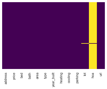
print(df.isnull().sum())

address        0
price          0
bed            0
bath           0
area           0
type           0
year_built     0
heating        0
cooling        0
parking        0
lot            1
hoa           97
url            0
dtype: int64

Data transformation

# drop column with too many missing values
df = df.drop(['hoa'], axis=1)

# drop remaining row with one missing value
df = df.dropna()

# Drop irrelevant features
df = df.drop(['url', 'address'], axis=1)

print(df.isnull().sum())

price         0
bed           0
bath          0
area          0
type          0
year_built    0
heating       0
cooling       0
parking       0
lot           0
dtype: int64

# Convert data types
categorical_list = ['type', 'heating', 'cooling', 'parking']

for i in categorical_list:
    df[i] = df[i].astype("category")

df.info()

<class 'pandas.core.frame.DataFrame'>
Int64Index: 97 entries, 0 to 97
Data columns (total 10 columns):
 #   Column      Non-Null Count  Dtype   
---  ------      --------------  -----   
 0   price       97 non-null     int64   
 1   bed         97 non-null     int64   
 2   bath        97 non-null     float64 
 3   area        97 non-null     int64   
 4   type        97 non-null     category
 5   year_built  97 non-null     int64   
 6   heating     97 non-null     category
 7   cooling     97 non-null     category
 8   parking     97 non-null     category
 9   lot         97 non-null     float64 
dtypes: category(4), float64(2), int64(4)
memory usage: 7.3 KB

# summary statistics for all categorical columns
df.describe(include=['category']).transpose()

	count	unique	top	freq
type	97	1	Single Family	97
heating	97	19	Forced air, Gas	34
cooling	97	2	other	52
parking	97	19	0 spaces	42

• Variable type has zero veriation (only single family) and therefore can be exluded from the analysis and the model.

• We will also exclude heatingand parking to keep this example as simple as possible.

df = df.drop(['type', 'heating', 'parking'], axis=1)
df

	price	bed	bath	area	year_built	cooling	lot
0	1520000	3	4.0	6040	1972	central	0.97
1	1030000	5	4.0	4475	1969	central	1.38
2	420000	2	3.0	1745	1959	central	0.51
3	680000	4	3.0	2091	1961	central	0.84
4	428500	4	3.0	1772	2020	central	0.16
...	...	...	...	...	...	...	...
93	541000	4	4.0	2740	1960	central	0.51
94	473000	3	3.0	2171	1955	other	0.61
95	490000	4	4.0	2972	1984	central	0.65
96	815000	4	4.0	3904	1970	other	1.47
97	674500	4	4.0	3766	1955	other	0.73

97 rows × 7 columns

Data splitting

train_dataset = df.sample(frac=0.8, random_state=0)
test_dataset = df.drop(train_dataset.index)

train_dataset

	price	bed	bath	area	year_built	cooling	lot
26	385000	3	2.0	1831	1951	central	0.29
85	485000	4	3.0	2609	1962	other	0.52
2	420000	2	3.0	1745	1959	central	0.51
55	150000	3	1.0	1734	1945	other	0.16
69	105000	2	1.0	1094	1940	other	0.26
...	...	...	...	...	...	...	...
96	815000	4	4.0	3904	1970	other	1.47
70	520000	4	3.0	2637	1968	other	0.65
20	270000	3	3.0	1416	1990	other	0.36
92	590000	5	3.0	3323	1980	other	0.43
73	592000	3	2.0	2378	1960	other	0.75

78 rows × 7 columns

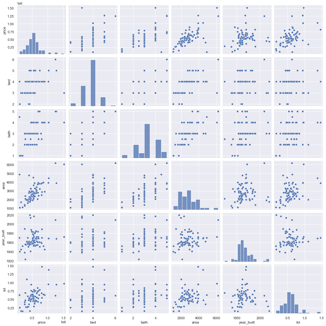
Exploratory data analysis

# summary statistics for all numerical columns
round(train_dataset.describe(),2).transpose()

	count	mean	std	min	25%	50%	75%	max
price	78.0	560762.18	243254.08	95000.00	421250.00	537500.00	650000.00	1520000.00
bed	78.0	3.81	0.74	2.00	3.00	4.00	4.00	6.00
bath	78.0	3.10	0.92	1.00	2.50	3.00	4.00	5.00
area	78.0	2831.40	986.38	1094.00	2095.25	2745.00	3261.75	6178.00
year_built	78.0	1965.82	16.80	1923.00	1956.25	1961.50	1971.50	2020.00
lot	78.0	0.59	0.23	0.15	0.45	0.56	0.69	1.47

sns.pairplot(train_dataset);

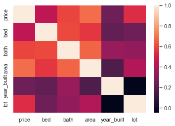
Correlation analysis

# Create correlation matrix for numerical variables
corr_matrix = train_dataset.corr()
corr_matrix

	price	bed	bath	area	year_built	lot
price	1.000000	0.446668	0.593686	0.680012	0.248102	0.537264
bed	0.446668	1.000000	0.599660	0.560258	0.216696	0.248166
bath	0.593686	0.599660	1.000000	0.659879	0.351917	0.335490
area	0.680012	0.560258	0.659879	1.000000	0.165495	0.412836
year_built	0.248102	0.216696	0.351917	0.165495	1.000000	-0.047352
lot	0.537264	0.248166	0.335490	0.412836	-0.047352	1.000000

# Simple heatmap
heatmap = sns.heatmap(corr_matrix)

# Make a pretty heatmap

# Use a mask to plot only part of a matrix
mask = np.zeros_like(corr_matrix)
mask[np.triu_indices_from(mask)]= True

# Change size
plt.subplots(figsize=(11, 15))

# Build heatmap with additional options
heatmap = sns.heatmap(corr_matrix, 
                      mask = mask, 
                      square = True, 
                      linewidths = .5,
                      cmap = 'coolwarm',
                      cbar_kws = {'shrink': .6,
                                'ticks' : [-1, -.5, 0, 0.5, 1]},
                      vmin = -1,
                      vmax = 1,
                      annot = True,
                      annot_kws = {"size": 10})

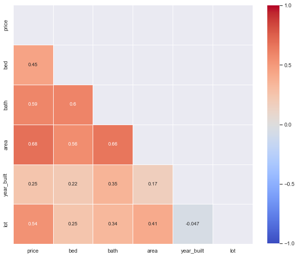
Instead of inspecting the correlation matrix, a better way to assess multicollinearity is to compute the variance inflation factor (VIF). Note that we ignore the intercept in this test.

• The smallest possible value for VIF is 1, which indicates the complete absence of collinearity.

• Typically in practice there is a small amount of collinearity among the predictors.

• As a rule of thumb, a VIF value that exceeds 5 indicates a problematic amount of collinearity and the parameter estimates will have large standard errors because of this.

Note that the function variance_inflation_factor expects the presence of a constant in the matrix of explanatory variables. Therefore, we use add_constant from statsmodels to add the required constant to the dataframe before passing its values to the function.

# choose features and add constant
features = add_constant(df[['bed', 'bath', 'area', 'lot']])
# create empty DataFrame
vif = pd.DataFrame()
# calculate vif
vif["VIF Factor"] = [variance_inflation_factor(features.values, i) for i in range(features.shape[1])]
# add feature names
vif["Feature"] = features.columns

vif.round(2)

	VIF Factor	Feature
0	28.52	const
1	1.74	bed
2	2.17	bath
3	2.14	area
4	1.19	lot

We don’t have a problematic amount of collinearity in our data.

Modeling

See separate notebooks.