Gradient Boosting in scikit-learn#
We illustrate the following regression method on a data set called “Hitters”, which includes 20 variables and 322 observations of major league baseball players. The goal is to predict a baseball player’s salary on the basis of various features associated with performance in the previous year. We don’t cover the topic of exploratory data analysis in this notebook.
Visit this documentation if you want to learn more about the data
Setup#
import matplotlib.pyplot as plt
import numpy as np

from sklearn.ensemble import GradientBoostingRegressor
from sklearn.metrics import mean_squared_error
from sklearn.inspection import permutation_importance
Data#
import pandas as pd
from sklearn.model_selection import train_test_split
from sklearn.preprocessing import StandardScaler

# Import
df = pd.read_csv("https://raw.githubusercontent.com/kirenz/datasets/master/Hitters.csv")

# drop missing cases
df = df.dropna()

# Create dummies
dummies = pd.get_dummies(df[['League', 'Division','NewLeague']])

# Create our label y:
y = df[['Salary']]
X_numerical = df.drop(['Salary', 'League', 'Division', 'NewLeague'], axis=1).astype('float64')

# Make a list of all numerical features
list_numerical = X_numerical.columns

# Create all features
X = pd.concat([X_numerical, dummies[['League_N', 'Division_W', 'NewLeague_N']]], axis=1)
feature_names = X.columns

# Split data
X_train, X_test, y_train, y_test = train_test_split(X, y, test_size=0.3, random_state=10)

# Data standardization
scaler = StandardScaler().fit(X_train[list_numerical])

X_train[list_numerical] = scaler.transform(X_train[list_numerical])
X_test[list_numerical] = scaler.transform(X_test[list_numerical])

# Make pandas dataframes
df_train = y_train.join(X_train)
df_test = y_test.join(X_test)
Make contiguous flattened arrays (for our scikit-learn GradientBoostingRegressor):
y_train = np.ravel(y_train)
y_test = np.ravel(y_test)
Model#
Define hyperparameters:
params = {
    "n_estimators": 500,
    "max_depth": 4,
    "min_samples_split": 5,
    "learning_rate": 0.01,
    "loss": "squared_error",
}
Build and fit model
Note
For big datasets (n_samples >= 10 000) the Histogram-based Gradient Boosting Regression Tree is much faster than GradientBoostingRegressor
reg = GradientBoostingRegressor(**params)

reg.fit(X_train, y_train)
GradientBoostingRegressor(learning_rate=0.01, max_depth=4, min_samples_split=5,
                          n_estimators=500)
In a Jupyter environment, please rerun this cell to show the HTML representation or trust the notebook. On GitHub, the HTML representation is unable to render, please try loading this page with nbviewer.org.
GradientBoostingRegressor(learning_rate=0.01, max_depth=4, min_samples_split=5,
                          n_estimators=500)
Make predictions
y_pred = reg.predict(X_test)
Evaluate model with RMSE
mean_squared_error(y_test, y_pred, squared=False)
302.26107555456184
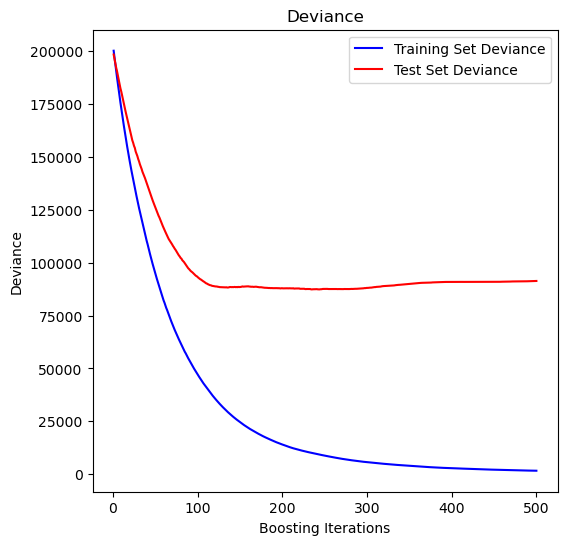
Plot training test deviance#
Source: scikit learn, provided by Peter Prettenhofer, Maria Telenczuk and Katrina Ni:
test_score = np.zeros((params["n_estimators"],), dtype=np.float64)

for i, y_pred in enumerate(reg.staged_predict(X_test)):
    test_score[i] = reg.loss_(y_test, y_pred)

fig = plt.figure(figsize=(6, 6))
plt.subplot(1, 1, 1)
plt.title("Deviance")
plt.plot(
    np.arange(params["n_estimators"]) + 1,
    reg.train_score_,
    "b-",
    label="Training Set Deviance",
)
plt.plot(
    np.arange(params["n_estimators"]) + 1, test_score, "r-", label="Test Set Deviance"
)
plt.legend(loc="upper right")
plt.xlabel("Boosting Iterations")
plt.ylabel("Deviance")
plt.show()
/Users/jankirenz/opt/anaconda3/envs/ds/lib/python3.9/site-packages/sklearn/utils/deprecation.py:103: FutureWarning: Attribute `loss_` was deprecated in version 1.1 and will be removed in 1.3.
  warnings.warn(msg, category=FutureWarning)
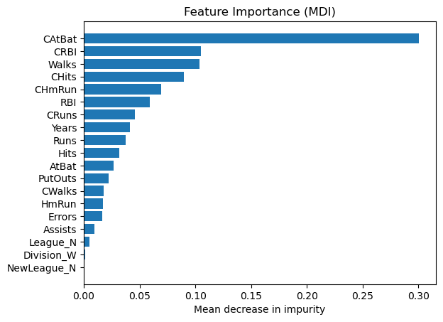
Feature importance#
Next, we take a look at the tree based feature importance and the permutation importance.
Mean decrease in impurity (MDI)#
Mean decrease in impurity (MDI) is a measure of feature importance for decision tree models.
Note
Visit this notebook to learn more about MDI
Feature importances are provided by the fitted attribute
feature_importances_
# obtain feature importance
feature_importance = reg.feature_importances_

# sort features according to importance
sorted_idx = np.argsort(feature_importance)
pos = np.arange(sorted_idx.shape[0])

# plot feature importances
plt.barh(pos, feature_importance[sorted_idx], align="center")

plt.yticks(pos, np.array(feature_names)[sorted_idx])
plt.title("Feature Importance (MDI)")
plt.xlabel("Mean decrease in impurity");
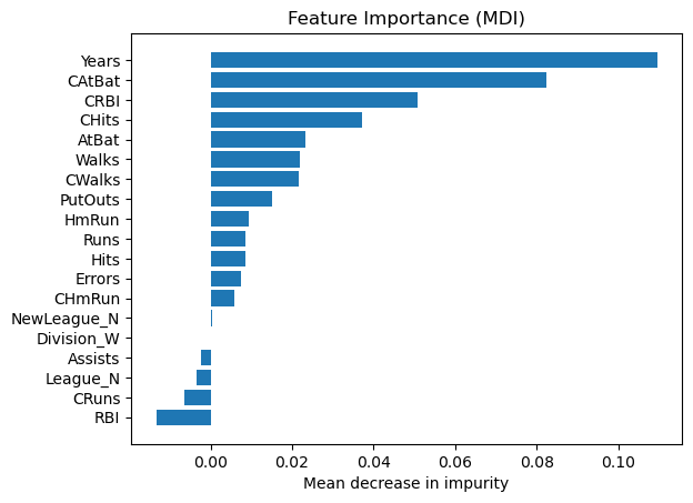
Permutation feature importance#
The permutation feature importance is defined to be the decrease in a model score when a single feature value is randomly shuffled.
Note
Visit this notebook to learn more about permutation feature importance.
result = permutation_importance(
    reg, X_test, y_test, n_repeats=10, random_state=42, n_jobs=2
)

tree_importances = pd.Series(result.importances_mean, index=feature_names)
# sort features according to importance
sorted_idx = np.argsort(tree_importances)
pos = np.arange(sorted_idx.shape[0])

# plot feature importances
plt.barh(pos, tree_importances[sorted_idx], align="center")

plt.yticks(pos, np.array(feature_names)[sorted_idx])
plt.title("Feature Importance (MDI)")
plt.xlabel("Mean decrease in impurity");
Same data plotted as boxplot:
plt.boxplot(
    result.importances[sorted_idx].T,
    vert=False,
    labels=np.array(feature_names)[sorted_idx],
)

plt.title("Permutation Importance (test set)")
Text(0.5, 1.0, 'Permutation Importance (test set)')
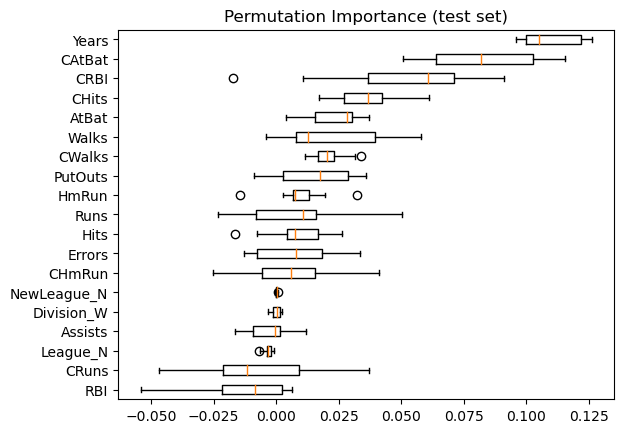
We observe that the same features are detected as most important using both methods (e.g.,
CAtBat,CRBI,CHits,Walks,Years). Although the relative importances vary (especially for featureYears).